Foreword
- Snippets and results.
- Source: 'Credit Risk Modeling with R' from DataCamp fitted into Jupyter/IPython, using the IRkernel.

Introduction to Data Structure
Exploring the credit data
Explore the data to get an idea of the number, and percentage, of defaults.
Banks make a profit from loaning to homeowners. Whenever a bank extends a mortgage loan, it takes a risk: the risk of default. In the data, a '1' represents a default, and a '0' represents non-default. A banks wants to minimize its risk exposure, therefore, minimize its expected losses.
$$ Expected~Loss = Probability~of~Default * Exposure~at~Default * Loss~given~Default $$First, import the data.
loan_data <- read.csv('loan_data.csv', header = TRUE, sep = ';')

# Or with
#loan_data2 <- read.table('loan_data.csv', header = TRUE, sep = ";")
Adjust the data.
loan_data$int_rate <- as.numeric(loan_data$int_rate) # variable is a factor
loan_data$annual_inc <- as.numeric(loan_data$annual_inc) # variable is a factor
loan_data$age <- as.integer(loan_data$age) # variable is a factor
Learn more about the variable structures and spot unexpected tendencies in the data.
# View the structure of loan_data
str(loan_data)
The CrossTable() function examines the relationship between loan_status (1 or 0) and certain factor variables.
Hypothesis: the proportion of defaults in the group of customers with grade G (worst credit rating score) should substantially be higher than the proportion of defaults in the grade A group (best credit rating score).
# Load the gmodels package
# Make sure the package is available for both RStudio and Jupyter
# install.packages('gmodels') in R
library(gmodels)

# Call CrossTable() on loan_status
CrossTable(loan_data$loan_status)
Notes on function CrossTable():
- x: A vector or a matrix. If y is specified, x must be a vector
- y: A vector in a matrix or a dataframe
- digits: Number of digits after the decimal point for cell proportions
- max.width: In the case of a 1 x n table, the default will be to print the output horizontally. If the number of columns exceeds max.width, the table will be wrapped for each successive increment of max.width columns. If you want a single column vertical table, set max.width to 1 expected If TRUE, chisq will be set to TRUE and expected cell counts from the χ2 will be included
- prop.r: If TRUE, row proportions will be included
- prop.c: If TRUE, column proportions will be included
- prop.t: If TRUE, table proportions will be included
- prop.chisq: If TRUE, chi-square contribution of each cell will be included
- chisq: If TRUE, the results of a chi-square test will be included
- fisher: If TRUE, the results of a Fisher Exact test will be included
- mcnemar: If TRUE, the results of a McNemar test will be included
- resid: If TRUE, residual (Pearson) will be included
- sresid: If TRUE, standardized residual will be included
- asresid: If TRUE, adjusted standardized residual will be included missing.include If TRUE, then remove any unused factor levels
- format: Either SAS (default) or SPSS, depending on the type of output desired.
- dnn: the names to be given to the dimensions in the result (the dimnames names).
- ...
# Call CrossTable() on grade and loan_status
CrossTable(loan_data$grade, loan_data$loan_status,
           prop.r = TRUE, # If TRUE, row proportions will be included
           prop.c = FALSE, # If TRUE, column proportions will be included
           prop.t = FALSE, # prop.t If TRUE, table proportions will be included
           prop.chisq = FALSE) # prop.chisq If TRUE, chi-square contribution of each cell will be included
Hypothesis confirmed: the proportion of defaults increases from Grade A (0.059) to Grade G (0.375).
Histograms
# Create histogram of loan_amnt: hist_1
hist_1 <- hist(loan_data$loan_amnt)

# Print locations of the breaks in hist_1
hist_1$breaks

# Change number of breaks and add labels
# Knowing the location of the breaks is important because
# if they are poorly chosen, the histogram may be misleading
hist_2 <- hist(loan_data$loan_amnt, breaks = 200, xlab = "Loan amount",
               main = "Histogram of the loan amount")

Note that there are some high peaks at round values: 5000, 10000, 15000, and so on because clients tend to borrow round numbers.
Ouliers
In the histogram above, there is a lot of blank space on the right-hand side of the plot. This is an indication of possible outliers.
If outliers are observed for several variables, it might be useful to look at bivariate plots. It's possible the outliers belong to the same observation.
A person with the huge annual wage of $6 million appeared to be 144 years old. This must be a mistake? Check it out.
# Plot the age variable
hist(loan_data$age, ylab = 'Frequency', main = 'Histogram of loan_data$age')

plot(loan_data$age, ylab = 'Age')

# Save the outlier's index to index_highage
index_highage <- which(loan_data$age > 122)

index_highage
# Make bivariate scatterplot of age and annual income
plot(loan_data$age, loan_data$annual_inc, xlab = "Age", ylab = "Annual Income")

# Create data set new_data with outlier deleted
new_data <- loan_data[-index_highage, ]
Missing data and coarse classification
How to deal with problematic data:
- delete the data
- replace the data
- keep the data
1. Deleting missing data
Some observations are missing interest rates. Identify how many rows are missing and delete them.
# Look at summary of loan_data (look for NA)
summary(loan_data$int_rate)
# Get indices of missing interest rates: na_index
na_index <- which(is.na(loan_data$int_rate))

# Remove observations with missing interest rates: loan_data_delrow_na
loan_data_delrow_na <- loan_data[-na_index, ]

summary(loan_data_delrow_na$int_rate)
# Make a copy of loan_data
loan_data_delcol_na <- loan_data

# Delete the interest rate column from loan_data_delcol_na
loan_data_delcol_na$int_rate <- NULL

summary(loan_data_delcol_na)
summary(loan_data)
2. Replacing missing data
- With continuous data: median imputation.
- With categorical data: most-frequent (category) imputation.
# Compute the median of int_rate
median_ir <- median(loan_data$int_rate, na.rm = TRUE)

# Make copy of loan_data
loan_data_replace <- loan_data

# Replace missing interest rates (na_index from above) with median
loan_data_replace$int_rate[na_index] <- median_ir

# Check if the NAs are gone
summary(loan_data_replace$int_rate)
3. Keeping the missing data
In some situations, the fact that an input is missing is an important information. NAs can be kept in a separate "missing" category using coarse classification.
Coarse classification requires to bin responses into groups that contain ranges of values. With this binning technique, place all NAs in their own bin.
# Make the necessary replacements in the coarse classification example below
# create the variable and fill it with NA
loan_data$ir_cat <- rep(NA, length(loan_data$int_rate))

loan_data$ir_cat[which(loan_data$int_rate <= 8)] <- "0-8"
loan_data$ir_cat[which(loan_data$int_rate > 8 & loan_data$int_rate <= 11)] <- "8-11"
loan_data$ir_cat[which(loan_data$int_rate > 11 & loan_data$int_rate <= 13.5)] <- "11-13.5"
loan_data$ir_cat[which(loan_data$int_rate > 13.5)] <- "13.5+"
loan_data$ir_cat[which(is.na(loan_data$int_rate))] <- "Missing"

loan_data$ir_cat <- as.factor(loan_data$ir_cat)

# Look at your new variable using plot()
plot(loan_data$ir_cat)

Data splitting and confusion matrices
First, start splitting the data into one training set (say 2/3) and one testing test (say 1/3). Second, use cross-validation splits (different train-test splits).
# Set seed of 567
set.seed(567)

# Store row numbers for training set: index_train
index_train <- sample(1:nrow(loan_data), 2 / 3 * nrow(loan_data))

# Create training set: training_set
training_set <- loan_data[index_train, ]

# Create test set: test_set
test_set <- loan_data[-index_train, ]

str(training_set)
str(test_set)
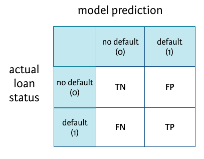
Creating a confusion matrix
Assume that you have run a model and stored the predicted outcomes in a vector called model_pred. In the next section, the focus is on logistic regression; a new topic.
See notes on machine learning for a complete coverage of these train-test techniques like decision or classification trees, random forests, knn, and an introduction to regressions.
See how the model performed with a confusion matrix.
R-code:
# Create confusion matrix
conf_matrix <- table(test_set$loan_status, model_pred)

# Compute classification accuracy
TN <- conf_matrix[1,1]
FP <- conf_matrix[1,2]
FN <- conf_matrix[2,1]
TP <- conf_matrix[2,2]
(TP+TN)/(TP+FP+TN+FN)

# Compute sensitivity
TP/(TP+FN)
Logistic Regression
Basic logistic regression or logit
It's a generalized linear model (GLM), as opposed to simple and multivariate linear regression (LM).
The former allows for different distributions of the data (such as the logistic distribution) while the later make the assumption the data are normally distributed.
In this GLM-Logit regression, the dependent variable is loan_status and age is the sole predictor.
# Build a glm model with variable ir_cat as a predictor
log_model_cat <- glm(loan_status ~ ir_cat, family = 'binomial', data = training_set)

# Print the parameter estimates
log_model_cat
# Look at the different categories in ir_cat using table()
table(loan_data$ir_cat)
# B0 and B1 per categories
log_model_cat$coefficients
log_model_cat$coefficients[1]
How do we interpret the parameter estimate for the interest rates that are between 8% and 11%?
B_0_8 <- as.numeric(log_model_cat$coefficients[1])
B_11_135 <- as.numeric(B_0_8 + log_model_cat$coefficients[2])
B_135 <- as.numeric(B_0_8 + log_model_cat$coefficients[3])
B_8_11 <- as.numeric(B_0_8 + log_model_cat$coefficients[4])
B_m <- as.numeric(B_0_8 + log_model_cat$coefficients[5])
$\beta$ < 0, default decreases as age increases (within the category):
B_0_8
B_8_11
The odds of defaulting decrease more with age (steeper negative curve) in 0-8% category than in the 8-11% category.
odds_0_8 <- exp(-2.88926885469467) # exp(B_0_8)
odds_8_11 <- exp(-2.30337633660622) # exp(B_8_11)
Probabilities of default: $e^{\beta} < 1$.
odds_0_8
odds_8_11
The odds of defaulting decrease as age increases (within the category).
As age goes up by 1, the odds increase by...
Compared to the reference category 0-8%, the odds of defaulting for category 8-11% change by a multiple of:
odds_8_11/odds_0_8
Multiple variables in a logistic regression model
The interpretation of a single parameter still holds when including several variables in a model.
When including several variables and asking for the interpretation when a certain variable changes, it is assumed that the other variables remain constant: ceteris paribus, literally meaning "keeping all others the same".
The significance of a parameter is often refered to as a p-value; denoted as $Pr(>|t|)$.
In a GLM,
- mild significance is denoted by a '
.', - very strong significance is denoted by '
***'.
When a parameter is not significant, you cannot assure the parameter is significantly different from 0.
# Build the logistic regression model
log_model_multi <- glm(loan_status ~
                       age + ir_cat + grade + loan_amnt + annual_inc,
                       family = 'binomial',
                       data = training_set)

# Obtain significance levels using summary()
summary(log_model_multi)
annual_inc is statistically significant where loan_amount is not.
Predicting the probability of default
Predict the probability for all the test set cases at once using the predict() function.
log_model_small <- glm(formula = loan_status ~ age + ir_cat,
                       family = "binomial", data = training_set)

summary(log_model_small)
# Build the logistic regression model
predictions_all_small <- predict(log_model_small, newdata = test_set, type = "response")

# Look at the range of the object "predictions_all_small"
format(range(predictions_all_small), trim = FALSE, digits = 3, nsmall = 2)
Looking at the range of predicted probabilities, a small range means that predictions for the test set cases do not lie far apart, and therefore the model might not be very good at discriminating good from bad customers.
The probability of default predictive model:
$$ P(loan\_status~=~1~|~age,~ir\_cat) = \frac{1}{1+e^{-(\hat{\beta_0}+\hat{\beta_1}*age+\hat{\beta_2}*ir\_cat)}} $$In the 0-8% category, the coefficient is the intercept without any adjustements (easy!)):
$$ P(loan\_status~=~1~|~age=33,~ir\_cat={[0-8]}) = \frac{1}{1+e^{-(-2.631128+(-0.009413)*33+0*1)}} $$Probability of default:
1 /
    (1 + exp(-1 *
         (as.numeric(log_model_small$coefficient[1]) +(as.numeric(log_model_small$coefficient[2]) * 33 + 0))))
Making more discriminative models
Small predicted default probabilities are to be expected with low default rates.
Building bigger models (which basically means: including more predictors) can expand the range of predictions.
First, transform the training_set and test-set: bin the emp_length variable, remove the emp_length and int_rate variables.
# Bin the `emp_length` variable
training_set_modified <- training_set
test_set_modified <- test_set

training_set_modified$emp_cat <- rep(NA, length(training_set$emp_length))
test_set_modified$emp_cat <- rep(NA, length(test_set$emp_length))

str(training_set_modified)
str(test_set_modified)
training_set_modified$emp_cat[which(training_set_modified$emp_length <= 15)] <- "0-15"
training_set_modified$emp_cat[which(training_set_modified$emp_length > 15 & training_set_modified$emp_length <= 30)] <- "15-30"
training_set_modified$emp_cat[which(training_set_modified$emp_length > 30 & training_set_modified$emp_length <= 45)] <- "30-45"
training_set_modified$emp_cat[which(training_set_modified$emp_length > 45)] <- "45+"
training_set_modified$emp_cat[which(is.na(training_set_modified$emp_length))] <- "Missing"

training_set_modified$emp_cat <- as.factor(training_set_modified$emp_cat)

# Look at your new variable using plot()
plot(training_set_modified$emp_cat)

test_set_modified$emp_cat[which(test_set_modified$emp_length <= 15)] <- "0-15"
test_set_modified$emp_cat[which(test_set_modified$emp_length > 15 & test_set_modified$emp_length <= 30)] <- "15-30"
test_set_modified$emp_cat[which(test_set_modified$emp_length > 30 & test_set_modified$emp_length <= 45)] <- "30-45"
test_set_modified$emp_cat[which(test_set_modified$emp_length > 45)] <- "45+"
test_set_modified$emp_cat[which(is.na(test_set_modified$emp_length))] <- "Missing"

test_set_modified$emp_cat <- as.factor(test_set_modified$emp_cat)

# Look at your new variable using plot()
plot(test_set_modified$emp_cat)

training_set_modified$emp_length <- NULL
test_set_modified$emp_length <- NULL
training_set_modified$int_rate <- NULL
test_set_modified$int_rate <- NULL

str(training_set_modified)
str(test_set_modified)
# Change the code below to construct a logistic regression model using all available predictors in the data set
#log_model_full <- glm(loan_status ~
#                      loan_status + loan_amnt + grade + home_ownership + annual_inc + age + emp_cat + ir_cat,
#                      family = "binomial",
#                      data = training_set2)

log_model_full <- glm(loan_status ~ .,
                      family = "binomial",
                      data = training_set_modified)

summary(log_model_full)
# Make PD-predictions for all test set elements using the the full logistic regression model
predictions_all_full <- predict(log_model_full, newdata = test_set_modified, type = "response")

# Look at the predictions range in percentage
format(range(predictions_all_full)*100, trim = FALSE, digits = 6, nsmall = 2)
Evaluating the logistic regression model results
Specify a cut-off (acceptance threshold). A good cut-off makes the difference to obtain a good confusion matrix.
# Make a binary predictions-vector using a cut-off of 15%
pred_cutoff_15 <- ifelse(predictions_all_full > 0.15, 1, 0) # more tolerant

# and of 20%
pred_cutoff_20 <- ifelse(predictions_all_full > 0.20, 1, 0) # less tolerant

pred_cutoff <- cbind(pred_cutoff_15, pred_cutoff_20)
head(pred_cutoff, 10)
# Make a binary predictions-vector using a cut-off of 15%
pred_cutoff_15 <- ifelse(predictions_all_full > 0.15, 1, 0)

# Construct a confusion matrix
table(test_set$loan_status, pred_cutoff_15)
# Check the length
str(test_set_modified)
str(predictions_all_full)
Construct a confusion matrix
pred_cutoff_15 <- ifelse(predictions_all_full > 0.15, 1, 0)
pred_cutoff_20 <- ifelse(predictions_all_full > 0.20, 1, 0)

conf_matrix_15 <- table(test_set_modified$loan_status, pred_cutoff_15)
conf_matrix_20 <- table(test_set_modified$loan_status, pred_cutoff_20)
$ Classification~Accuracy = \frac{(TP+TN)}{(TP+FP+TN+FN)} $
$ Classification~Sensitivity = \frac{TP}{(TP+FN)} $
$ Classification~Specificity = \frac{TN}{(FP+TN)} $
# Compute classification accuracy
TN <- conf_matrix_15[1,1]
FP <- conf_matrix_15[1,2]
FN <- conf_matrix_15[2,1]
TP <- conf_matrix_15[2,2]

# Compute accuracy
A_15 <- (TP + TN) / (TP + FP + TN + FN)
A_15

# Compute sensitivity
S_15 <- TP / (TP + FN)
S_15

# Compute specificity
Sp_15 <- TN / (FP + TN)
Sp_15
# Compute classification accuracy
TN <- conf_matrix_20[1,1]
FP <- conf_matrix_20[1,2]
FN <- conf_matrix_20[2,1]
TP <- conf_matrix_20[2,2]

# Compute accuracy
A_20 <- (TP + TN) / (TP + FP + TN + FN)
A_20

# Compute sensitivity
S_20 <- TP / (TP + FN)
S_20

# Compute specificity
Sp_20 <- TN / (FP + TN)
Sp_20
Moving from a cut-off of 15% to 20%: accuracy increases, sensitivity decreases and specificity increases.
Pointer: performing simulations with loops would enable the graphing of the results on a cut-off range (0 to 100%).
Alternative models
The model used so far: glm(loan_status ~ .,family = "binomial", data = training_set2)
By default, the attribute is set on family = "binomial"(link = logit), but there are other types of models such as family = "binomial"(link = probit) and family = "binomial"(link = cloglog).
They behave like the logit model, but their specifications are more complex.
# Fit the logit, probit and cloglog-link logistic regression models
log_model_logit <- glm(loan_status ~ age + emp_cat + ir_cat + loan_amnt,
                       family = binomial(link = logit), data = training_set_modified)

log_model_probit <- glm(loan_status ~ age + emp_cat + ir_cat + loan_amnt,
                       family = binomial(link = probit), data = training_set_modified)

log_model_cloglog <- glm(loan_status ~ age + emp_cat + ir_cat + loan_amnt,
                       family = binomial(link = cloglog), data = training_set_modified)
summary(log_model_logit)
summary(log_model_probit)
summary(log_model_cloglog)
# Make predictions for all models using the test set
predictions_logit <- predict(log_model_logit,
                             newdata = test_set_modified,
                             type = "response")
predictions_probit <- predict(log_model_probit,
                              newdata = test_set_modified,
                              type = "response")
predictions_cloglog <- predict(log_model_cloglog,
                               newdata = test_set_modified,
                               type = "response")
Use the predict() on GLM:
http://stat.ethz.ch/R-manual/R-patched/library/stats/html/predict.glm.html
# Use a cut-off of 14% to make binary predictions-vectors
cutoff <- 0.14

true_value <- test_set_modified$loan_status
class_pred_logit <- ifelse(predictions_logit > cutoff, 1, 0)
class_pred_probit <- ifelse(predictions_probit > cutoff, 1, 0)
class_pred_cloglog <- ifelse(predictions_cloglog > cutoff, 1, 0)

class_pred <- cbind(true_value, class_pred_logit, class_pred_probit, class_pred_cloglog)
head(class_pred, 20)
str(true_value)
str(class_pred_logit)
# Make a confusion matrix for the three models
tab_class_logit <- table(true_value, class_pred_logit)
tab_class_probit <- table(true_value, class_pred_probit)
tab_class_cloglog <- table(true_value, class_pred_cloglog)

tab_class_logit
tab_class_probit
tab_class_cloglog
# Compute the classification accuracy for all three models
acc_logit <- sum(diag(tab_class_logit)) / nrow(test_set_modified)
acc_probit <- sum(diag(tab_class_probit)) / nrow(test_set_modified)
acc_cloglog <- sum(diag(tab_class_cloglog)) / nrow(test_set_modified)

acc_logit * 100
acc_probit * 100
acc_cloglog * 100
The three models yield the same results (given they all are predictive models and there is a certain margin of error involved).

Decision Trees
Computing the gain for a tree
The Gini-measure is used to create the perfect split for a tree.
The data set contains 500 cases, 89 of these cases are defaults. This led to a Gini of 0.292632 in the root node.
The Gini of a:
$$ certain~node = 2 * proportion~of~defaults * proportion~of~nondefaults $$gini_root <- 2 * (89 / 500) * (411 / 500)
Use these Gini measures to calculate the gain of the leaf nodes with respect to the root node.
Gain <-
    gini_root -
    (prop(cases left leaf) * gini_left) -
    (prop(cases right leaf * gini_right))

# The Gini-measure of the root node is given below (89 + 411 = 500)
gini_root <- 2 * 89 / 500 * 411 / 500
gini_root

# Compute the Gini measure for the left leaf node (401 + 45 = 446)
gini_ll <- 2 * 401 / 446 * 45 / 446
gini_ll

# Compute the Gini measure for the right leaf node (10 + 44 = 54)
gini_rl <- 2 * 10 / 54 * 44 / 54
gini_rl

# Compute the gain
gain <- gini_root - 446 / 500 * gini_ll - 54 / 500 * gini_rl
gain
Compare the gain-column in small_tree$splits with our computed gain, multiplied by 500, and assure they are the same (for now, the small_tree object is not calculated):
small_tree$splits

    count ncat  improve index adj
age   500    1 49.10042  32.5   0
improve <- gain * 500
improve
How would a change in the right leaf proportions from 10/44 to 20/34 change the gain?
# The Gini-measure of the root node is given below (89 + 411 = 500)
gini_root <- 2 * 89 / 500 * 411 / 500
gini_root

# Compute the Gini measure for the left leaf node (401 + 45 = 446)
gini_ll <- 2 * 401 / 446 * 45 / 446
gini_ll

# HERE
# Compute the Gini measure for the right leaf node (20 + 34 = 54)
gini_rl <- 2 * 20 / 54 * 34 / 54
gini_rl

# Compute the gain
gain <- gini_root - 446 / 500 * gini_ll - 54 / 500 * gini_rl
gain
The gain would go down from 0.10 to 0.80.
Building decision trees using the rpart package
But, it is hard building nice decision tree for credit risk data because of unbalanced data.
Overcome the unbalance:
- Undersampling or oversampling
- Accuracy issue will disappear
- Only training set
- Changing the prior probabilities
- Including a loss matrix
1. Undersampling the training set
Under- or oversampling. The training set is undersampled, such that after transformation, 1/3 of the training set consists of defaults, and 2/3 of non-defaults (undersampling defaulting).
# Import the data
undersampled_training_set <- read.csv('undersampled_training_set.csv', header = TRUE, sep = ';')

#true_val <- true_val$true_value
str(undersampled_training_set)
# Load package rpart() in your workspace.
library(rpart)
# Change the code provided in the video such that a decision tree is constructed using the undersampled training set.
# If cp is not met, further splits will no longer be pursued. cp's default value is 0.01, but for complex problems, it is advised to relax cp to 0.001.
tree_undersample <- rpart(loan_status ~ ., method = "class",
                          data =  undersampled_training_set,
                          control = rpart.control(cp = 0.001))

# Plot the decision tree; uniform for equal-size branches
plot(tree_undersample, uniform = TRUE)

# Add labels to the decision tree
text(tree_undersample)

Mmmm... a bit crowded.
2. Changing the prior probabilities
With argument: parms = list(prior = c(non_default_proportion, default_proportion)), using the complete training set.
# Change the code below such that a tree is constructed with adjusted prior probabilities.
# parms = list(prior=c(non_default_proportion, default_proportion))
tree_prior <- rpart(loan_status ~ ., method = "class",
                    data = training_set_modified,
                    parms = list(prior = c(0.7, 0.3)),
                    control = rpart.control(cp = 0.001))

# Plot the decision tree
plot(tree_prior, uniform = TRUE)

# Add labels to the decision tree
text(tree_prior)

3. Including a loss matrix
Change the relative importance of misclassifying a default as non-default versus a non-default as a default. Stress that misclassifying a default as a non-default should be penalized more heavily.
Use argument: parms = list(loss = matrix(c(0, cost_def_as_nondef, cost_nondef_as_def, 0), ncol=2)).
# Change the code below such that a decision tree is constructed
# using a loss matrix penalizing 10 times more heavily for misclassified defaults.
# parms = list(loss = matrix(c(0, cost_def_as_nondef, cost_nondef_as_def, 0), ncol=2))
tree_loss_matrix <- rpart(loan_status ~ ., method = "class",
                    data = training_set_modified,
                    parms = list(loss = matrix(c(0, 10, 1, 0), ncol=2)),
                    control = rpart.control(cp = 0.001))

# Plot the decision tree
plot(tree_loss_matrix, uniform = TRUE)

# Add labels to the decision tree
text(tree_loss_matrix)

Pruning the decision tree
Pruning a tree is necessary to avoid overfitting (as above).
Use printcp() and plotcp() for pruning purposes.
library(rpart.plot)
tree_prior from Changing the prior probabilities
# Use printcp() to identify for which complexity parameter the cross-validated error rate is minimized.
printcp(tree_prior)
# Plot the cross-validated error rate as a function of the complexity parameter
plotcp(tree_prior)

# Create an index for of the row with the minimum xerror
index <- which.min(tree_prior$cptable[ , "xerror"])
index

# Create tree_min
tree_min <- tree_prior$cptable[index, "CP"]
tree_min
#  Prune the tree using tree_min
ptree_prior <- prune(tree_prior, cp = tree_min)

# Use prp() to plot the pruned tree
prp(ptree_prior, extra = 1)

tree_loss_matrix from Including a loss matrix
tree_loss_matrix <- rpart(loan_status ~ ., method = "class",
                    data = training_set_modified,
                    parms = list(loss = matrix(c(0, 10, 1, 0), ncol=2)),
                    control = rpart.control(cp = 0.001))

# Use printcp() to identify for which complexity parameter the cross-validated error rate is minimized.
printcp(tree_loss_matrix)
# Plot the cross-validated error rate as a function of the complexity parameter
plotcp(tree_loss_matrix)

# Create an index for of the row with the minimum xerror
index <- which.min(tree_loss_matrix$cptable[ , "xerror"])
index

# Create tree_min
tree_min <- tree_prior$cptable[index, "CP"]
tree_min
# Prune the tree (using the above cp will be too much)
# on the graph above, the error touches the asymptote for the first time
ptree_loss_matrix <- prune(tree_loss_matrix, cp = 0.0014)

# Use prp() and argument extra = 1 to plot the pruned tree
prp(ptree_loss_matrix, extra = 1)

tree_undersampled from Undersampling the training set
# Use printcp() to identify for which complexity parameter the cross-validated error rate is minimized.
printcp(tree_undersample)
plotcp(tree_undersample)

index <- which.min(tree_undersample$cptable[ , "xerror"])
index

tree_min <- tree_undersample$cptable[index, "CP"]
tree_min
# take the second minimum or 5th position where cp = 0.0029680
ptree_undersample <- prune(tree_undersample, cp = 0.0029680)

prp(ptree_undersample, extra = 1)

One final tree using more options
Case weights
This vector contains weights of 1 for the non-defaults in the training set, and weights of 3 for defaults in the training sets. By specifying higher weights for default, the model will assign higher importance to classifying defaults correctly.
# Import the data
training_set2 <- read.csv('training_set2.csv', header = TRUE, sep = ';')
case_weights <- read.csv('case_weights.csv', header = TRUE, sep = ';')
str(training_set2)
case_weights <- as.numeric(case_weight$case_weights)
str(case_weights)
class(case_weights)
# set a seed and run the code to obtain a tree using weights, minsplit and minbucket
set.seed(345)
tree_weights <- rpart(loan_status ~ ., method = "class",
                      data = training_set2, weights = case_weights,
                      control = rpart.control(minsplit = 5, minbucket = 2, cp = 0.001))
printcp(tree_weights)
# Plot the cross-validated error rate for a changing cp
plotcp(tree_weights)

# Create an index for of the row with the minimum xerror
index <- which.min(tree_weights$cp[ , "xerror"])
index

# Create tree_min
tree_min <- tree_weights$cp[index, "CP"]
tree_min
# Prune the tree using tree_min
ptree_weights <- prune(tree_weights, cp = tree_min)

# Plot the pruned tree using the rpart.plot()-package
prp(ptree_weights, extra = 1)

Confusion matrices and accuracy of our final trees
The number of splits varies quite a bit from one tree to another:
| Tree | Obs | CP | Splits |
|---|---|---|---|
| ptree_prior | 19394 | 0.0035 | 7 |
| ptree_loss_matrix | 19394 | 0.0025 | 26 |
| ptree_loss_undersample | 6570 | 0.0030 | 11 |
| ptree_weight | 19394 | 0.0010 | 7 |
Make predictions using the test set.
test_set_modified <- read.csv('test_set_modified.csv', header = TRUE, sep = ';')
# Make predictions for each of the pruned trees using the test set.
pred_prior <- predict(ptree_prior,
                            newdata = test_set_modified,
                            type = "class")

pred_loss_matrix <- predict(ptree_loss_matrix,
                            newdata = test_set_modified,
                            type = "class")

pred_undersample <- predict(ptree_undersample,
                            newdata = test_set_modified,
                            type = "class")

pred_weights <- predict(ptree_weights,
                            newdata = test_set_modified,
                            type = "class")
pred_prior <- as.numeric(as.character(pred_prior))
pred_loss_matrix <- as.numeric(as.character(pred_loss_matrix))
pred_undersample <- as.numeric(as.character(pred_undersample))
pred_weights <- as.numeric(as.character(pred_weights))
Use predict() on trees: http://stat.ethz.ch/R-manual/R-patched/library/rpart/html/predict.rpart.html
pred_loss_matrix3 <- predict(ptree_loss_matrix,
                            newdata = test_set_modified,
                            type = "prob")
head(pred_loss_matrix3)
head(pred_loss_matrix3[,2])
head(predictions_cloglog)
Construct the confusion matrix for each of these trees.
Nevertheless, it is important to be aware of the fact that not only the accuracy is important, but also the sensitivity and specificity.
$ Classification~Accuracy = \frac{(TP+TN)}{(TP+FP+TN+FN)} $
$ Classification~Sensitivity = \frac{TP}{(TP+FN)} $
$ Classification~Specificity = \frac{TN}{(FP+TN)} $
# construct confusion matrices using the predictions.
confmat_prior <- table(test_set_modified$loan_status, pred_prior)
confmat_loss_matrix <- table(test_set_modified$loan_status, pred_loss_matrix)
confmat_undersample <- table(test_set_modified$loan_status, pred_undersample)
confmat_weights <- table(test_set_modified$loan_status, pred_weights)

# Compute the accuracies
acc_prior <- sum(diag(confmat_prior)) / nrow(test_set_modified)
acc_loss_matrix <- sum(diag(confmat_loss_matrix)) / nrow(test_set_modified)
acc_undersample <- sum(diag(confmat_undersample)) / nrow(test_set_modified)
acc_weights <- sum(diag(confmat_weights)) / nrow(test_set_modified)

acc_prior
acc_loss_matrix
acc_undersample
acc_weights
ptree_prior and ptree_undersample are good predictor. ptree_weight is the best model.

Evaluating a Credit Risk Model
Computing a bad rate given a fixed acceptance rate
Compute the bad rate that a bank can expect (the cut-off) when using the pruned tree ptree_prior that you fitted before, and an acceptance rate of 80% given the tree below.
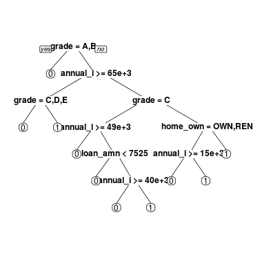
# Make predictions for the probability of default using the pruned tree and the test set.
prob_default_prior <- predict(ptree_prior, newdata = test_set_modified)[ ,2]

head(prob_default_prior, 10)
# Obtain the cutoff for acceptance rate 80%
cutoff_prior <- quantile(prob_default_prior, 0.80)

cutoff_prior
# Obtain the binary predictions.
bin_pred_prior_80 <- ifelse(prob_default_prior > cutoff_prior, 1, 0)

head(bin_pred_prior_80, 10)

# where the prob_default_prior > cutoff_prior,
# the bin_pred_default_prior yields 1 or aprediction of default
# Obtain the actual default status for the accepted loans
accepted_status_prior_80 <- test_set_modified$loan_status[bin_pred_prior_80 == 0]

head(cbind(bin_pred_prior_80, accepted_status_prior_80), 10)
# Obtain the bad rate for the accepted loans
sum(accepted_status_prior_80) / length(accepted_status_prior_80)
The strategy table and strategy curve
This table is a useful tool for banks, as they can give them a better insight to define an acceptance strategy.
predictions_cloglog should be obtained from section 2 (extract the probabilities from the results)...
head(predictions_cloglog)
strategy_bank <- function(prob_of_def) {
    cutoff = rep(NA, 21)
    bad_rate = rep(NA, 21)
    accept_rate = seq(1,0,by = -0.05)

    for (i in 1:21){
        cutoff[i] = quantile(prob_of_def, accept_rate[i])
        pred_i = ifelse(prob_of_def > cutoff[i], 1, 0)
        pred_as_good = test_set$loan_status[pred_i==0]
        bad_rate[i] = sum(pred_as_good) / length(pred_as_good)
    }
    table = cbind(accept_rate, cutoff=round(cutoff,4), bad_rate = round(bad_rate,4))

    return(list(table = table,
                bad_rate = bad_rate,
                accept_rate = accept_rate,
                cutoff = cutoff))
}
# need the probability of default (1)
head(predictions_cloglog)

pred_loss_matrix2 <- predict(ptree_loss_matrix,
                            newdata = test_set_modified,
                            type = "prob")
head(pred_loss_matrix2)
head(pred_loss_matrix2[,2])
predictions_loss <- pred_loss_matrix2[,2]
# Apply the function strategy_bank to both predictions_cloglog and predictions_loss_matrix
strategy_cloglog <- strategy_bank(predictions_cloglog)

strategy_loss_matrix <- strategy_bank(predictions_loss)
# Obtain the strategy tables for both prediction-vectors
strategy_cloglog$table
strategy_loss_matrix$table
Keep in mind that a pruned tree model depends on the datasets and the cp coefficient... The next graph can vary a lot depending on these two factors.
# Plot the strategy functions
par(mfrow = c(1,2))

plot(strategy_cloglog$accept_rate, strategy_cloglog$bad_rate,
     type = "l", xlab = "Acceptance rate", ylab = "Bad rate",
     lwd = 2, main = "logistic regression")

plot(strategy_loss_matrix$accept_rate, strategy_loss_matrix$bad_rate,
     type = "l", xlab = "Acceptance rate",
     ylab = "Bad rate", lwd = 2, main = "tree")

This is what another pruned tree model produced:

Based on the last set of plots, if:
- Bank A has to use an acceptance rate of 45%.
- Bank B has to use an acceptance rate of 85%.
To minimize the 'Bad rate':
- Bank A would prefer the tree model.
- Bank B would prefer the logistic regression model.
ROC-curves for comparison of logistic regression models
ROC-curves are created using the pROC-package.
# Load the pROC-package
library(pROC)
# Construct the objects containing ROC-information
# from section 2
# roc(response, predictor)
# response is the loan status indicator in the test_set
ROC_logit <- roc(test_set_modified$loan_status, predictions_logit)
ROC_probit <- roc(test_set_modified$loan_status, predictions_probit)
ROC_cloglog <- roc(test_set_modified$loan_status, predictions_cloglog)
ROC_all_full <- roc(test_set_modified$loan_status, predictions_all_full)
# Draw all ROCs on one plot
plot(ROC_logit)

lines(ROC_probit, col= 'blue')
lines(ROC_cloglog, col= 'red')
lines(ROC_all_full, col= 'green')

# Compute the AUCs
auc(ROC_logit)
auc(ROC_probit)
auc(ROC_cloglog)
auc(ROC_all_full)
ROC-curves for comparison of tree-based models
Repreat the comparison for the tree-based models.
# Construct the objects containing ROC-information
# roc(response, predictor)
ROC_undersample <- roc(test_set_modified$loan_status, pred_undersample)
ROC_prior <- roc(test_set_modified$loan_status, pred_prior)
ROC_loss_matrix <- roc(test_set_modified$loan_status, pred_loss_matrix)
ROC_weights <- roc(test_set_modified$loan_status, pred_weights)
# Draw the ROC-curves in one plot
plot(ROC_undersample)

lines(ROC_prior, col= 'blue')
lines(ROC_loss_matrix, col= 'red')
lines(ROC_weights, col= 'green')

# Compute the AUCs
auc(ROC_undersample)
auc(ROC_prior)
auc(ROC_loss_matrix)
auc(ROC_weights)
Another round of pruning based on AUC
The variable home_ownership was deleted from the model, as it improved the overall AUC. After repeating this process for two additional rounds, the variables age and ir_cat were deleted, leading to the model:
log_3_remove_ir <- glm(loan_status ~ loan_amnt + grade + annual_inc + emp_cat, family = binomial, data = training_set)
with an AUC of 0.6545. Now, it's your turn to see whether the AUC can still be improved by deleting another variable from the model.
# Build four models each time deleting one variable in log_3_remove_ir
log_4_remove_amnt <- glm(loan_status ~ grade + annual_inc + emp_cat,
                         family = binomial, data = training_set_modified)

log_4_remove_grade <- glm(loan_status ~ loan_amnt  + annual_inc + emp_cat,
                          family = binomial, data = training_set_modified)

log_4_remove_inc <- glm(loan_status ~ loan_amnt + grade  + emp_cat ,
                        family = binomial, data = training_set_modified)

log_4_remove_emp <- glm(loan_status ~ loan_amnt + grade + annual_inc,
                        family = binomial, data = training_set_modified)
# Make PD-predictions for each of the models
pred_4_remove_amnt <- predict(log_4_remove_amnt, newdata = test_set_modified, type = "response")
pred_4_remove_grade <- predict(log_4_remove_grade, newdata = test_set_modified, type = "response")
pred_4_remove_inc <- predict(log_4_remove_inc, newdata = test_set_modified, type = "response")
pred_4_remove_emp <- predict(log_4_remove_emp, newdata = test_set_modified, type = "response")
# Compute the AUCs
auc(test_set_modified$loan_status, pred_4_remove_amnt)
auc(test_set_modified$loan_status, pred_4_remove_grade)
auc(test_set_modified$loan_status, pred_4_remove_inc)
auc(test_set_modified$loan_status, pred_4_remove_emp)
log_4_remove_amnt is the best model for the area under the curve AUC.
Further model reduction?
Deleting the variable loan_amnt, the AUC can be further improved to 0.6548! The resulting model is:
log_4_remove_amnt <- glm(loan_status ~ grade + annual_inc + emp_cat, family = binomial, data = training_set)
Is it possible to reduce the logistic regression model to only two variable without reducing the AUC?
# Build three models each time deleting one variable in log_4_remove_amnt
log_5_remove_grade <- glm(loan_status ~ annual_inc + emp_cat, family = binomial, data = training_set_modified)
log_5_remove_inc <- glm(loan_status ~ grade  + emp_cat , family = binomial, data = training_set_modified)
log_5_remove_emp <- glm(loan_status ~ grade + annual_inc, family = binomial, data = training_set_modified)
# Make PD-predictions for each of the models
pred_5_remove_grade <- predict(log_5_remove_grade, newdata = test_set_modified, type = "response")
pred_5_remove_inc <- predict(log_5_remove_inc, newdata = test_set_modified, type = "response")
pred_5_remove_emp <- predict(log_5_remove_emp, newdata = test_set_modified, type = "response")
# Compute the AUCs
auc(test_set_modified$loan_status, pred_5_remove_grade)
auc(test_set_modified$loan_status, pred_5_remove_inc)
auc(test_set_modified$loan_status, pred_5_remove_emp)
# Plot the ROC-curve for the best model here
plot(roc(test_set_modified$loan_status, pred_4_remove_amnt))

log_4_remove_amnt still is the best model for the area under the curve AUC.

Conclusion
Other methods for predicting the risk of defaulting:
- Discriminant analysis
- Random forest
- Neural networks
- Support vector machines
But, the timing aspect is neglected in all the above methods (including logistic regressions and decision/classification trees).
A new popular method is survival analysis.
Survival analysis models the probability of default that change over time. Time-varying covariates can be included.